41 Context-Free Grammars
(defn logsumexp [& log-vals]
  (let [mx (apply max log-vals)]
    (+ mx
       (Math/log2
	     (apply +
	       (map (fn [z] (Math/pow 2 z))
		    (map (fn [x] (- x mx))
			log-vals)))))))

(defn flip [p]
  (if (< (rand 1) p)
    true
    false))

(defn score-categorical [outcome outcomes params]
  (if (empty? params)
    (throw "no matching outcome")
    (if (= outcome (first outcomes))
     (Math/log2 (first params))
      (score-categorical outcome (rest outcomes) (rest params)))))

(defn list-unfold [generator len]
  (if (= len 0)
    '()
    (cons (generator)
    (list-unfold generator (- len 1)))))


(defn sample-gamma [shape scale]
(apply + (repeatedly
  shape  (fn []
		     (- (Math/log2 (rand))))
		)))

(defn sample-dirichlet [pseudos]
  (let [gammas (map (fn [sh]
                     (sample-gamma sh 1))
                pseudos)]
    (normalize gammas)))

(defn normalize [dist]
  (let [sum (apply + (map prob dist))]
    (map
     (fn [x]
       [(value x) (/ (prob x) sum)] )
     dist)))

(defn sample-categorical [dist]
  (if (flip (prob (first dist)))
    (value (first dist))
    (sample-categorical
     (normalize (rest dist)))))
The standard formalism introduced to handle the kinds of structure discussed in the last lecture are known as context-free grammars for reason which we will cover in a later lecture. The basic idea behind a context-free grammar is that we will start with a new kind of object a lexicon. The lexicon is a set of words from a vocabulary, together with the category and argument structure requirements of those words.
A lexical item will consist of three kinds of information
- The category of the head word.
- The categories of the dependent phrases.
- The positions of the dependent phrases with respect to the head and one another.
Let’s use a Clojure record to implement lexical items.
(defrecord li [cat deps])

(li. :V [:N 'loves :N])
A lexical item is a record with two fields. The first is the category of the lexical item. The second is a list of dependents as well as the lexical item itself, all in the order in which they appear in the string. In context-free grammar terminology, words from the vocabulary are called terminals since they terminate computation, while categories are called nonterminals.
Note that our definition of a lexical item will allow us to introduce lexical items with more than one terminal. This might be useful for defining lexical items corresponding to idioms.
(li. :V [:N 'kick 'the 'bucket])
The definition also allows us to define lexical items without any terminals (or equivalently, \(\epsilon\) terminals). This can be useful if we wish, for instance to allow there to be null-head category converting rules.
(li. :V [:N])
I can also be used to implement the rule that combines a subject and a predicate to form a sentence (a so-called exocentric or non-headed structure, according to some accounts).
(li. :S [:N :V])
A lexicon is a set of such lexical items, together with probabilities for each lexical item, such that the probabilities form a set of conditional distributions—one for each category of item.
(defn prob [outcome]
  (second outcome))

(defn value [outcome]
  (first outcome))

(def lexicon
{:S  (list
	   [(li. :S [:N :V]) (/ 1 1)])

	:V  (list
	   [(li. :V ['loves :N]) (/ 1 2)]
	   [(li. :V ['calls :N]) (/ 1 2)])
      :N (list
	  [(li. :N ['John]) (/ 1 3)]
	  [(li. :N ['Fred]) (/ 1 3)]
	  [(li. :N ['Mary]) (/ 1 3)])})

(defn sample-li [lexicon cat]
  (sample-categorical (lexicon cat)))

(sample-li lexicon :S)
Now we are prepared to give the generative model for context-free grammars, which looks like this.
(def terminal? symbol?)
(defn tree-unfold [lexicon sym]
(if (terminal? sym)
sym
(into [sym]
(map (fn [s] (tree-unfold lexicon s))
(:deps (sample-li lexicon sym))))))
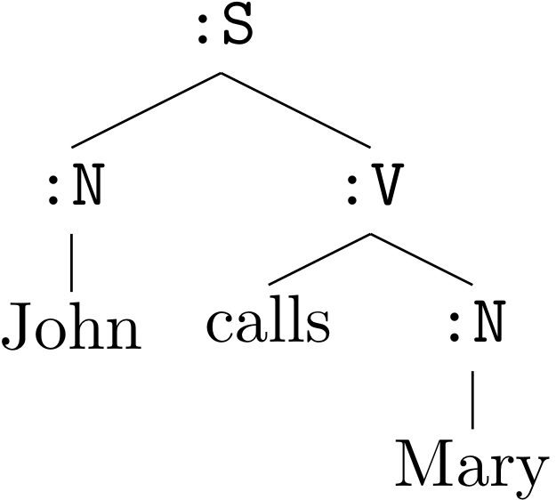
(tree-unfold lexicon :S)
This call to tree-unfold has printed a derivation or parse tree in context-free grammar terminology, indicating the way in which the sentence was built using the lexicon. We often draw such derivations as trees.
Formalizing Context-Free Grammars
Formally, a CFG is a 4-tuple, \(\mathcal{G}= \langle N_{\mathcal{G}}, V_{\mathcal{G}}, R_{\mathcal{G}}, \mathtt{S}\rangle\)
- \(N_{\mathcal{G}}\) is a finite set of nonterminal symbols.
- \(V_{\mathcal{G}}\) is a finite set of terminal symbols (distinct from \(V_{\mathcal{G}}\)).
- \(R_{\mathcal{G}} \subseteq V_{\mathcal{G}} \times (V_{\mathcal{G}} \cup T_{\mathcal{G}})^*\) is a finite set of production rules.
- S \(\ in V_{\mathcal{G}}\) is a unique, distinguished start symbol.
By convention, nonterminals are written with capital letters, and, when used to model linguistic structure, they represent categories of constituents such as, verb (V) or noun (N). The unique, distinguished nonterminal known as the start symbol is written S (for sentence). This symbol represents the category of complete derivations: sentences for syntax. Terminal symbols, written here in italics, typically represent atomic words or morphemes.
Production rules are written \(\mathtt{A} \longrightarrow \gamma\), where \(\gamma\) is some sequence of terminals and nonterminals, and A is a nonterminal. The set of production rules defines the possible computations for a CFG. For example, the rule, \(\mathtt{NP} \longrightarrow \mathtt{Det}\ \mathtt{N}\), says that a constituent of type N can be constructed by first constructing an adjective Det, and then a N and concatenating them together. The list of symbols to the right of the arrow is referred to as the right-hand side of that rule. The nonterminal to the left of the arrow is the rule’s left-hand side. The functions \(\mathrm{lhs}(r)\) and \(\mathrm{rhs}(r)\) return the left-hand side and right-hand side of rule \(r\), respectively. The language \(\mathcal{L}_{\mathtt{A}}\) associated with nonterminal A is the set of expressions that can be derived from that nonterminal by recursive application of the production rules of the grammar. The language associated with a CFG \(\mathcal{G}\) is \(\mathcal{L}_{\mathtt{S}}\) .
Categorical Probabilistic Context-Free Grammars
A categorical distribution is the simplest way of specifying a distribution over a finite number of discrete choices. If there are \(K\) possible choices, we simply specify a vector of probabilities of length \(K\) (i.e., a vector of real numbers \(\vec{\theta}\), such that \(\theta_i \geq 0\) and \(\sum_i \theta_i = 1\)). A multinomial PCFG is the simplest version of a probabilistic CFG, where the distributions over rule choices are given by multinomial distributions.
A derivation or parse tree is a tree representing the trace of the computation of some expression \(\vec{w}\), beginning from some nonterminal category A. A derivational tree is complete if all of its leaves are terminal symbols. A derivation tree fragment is a derivation tree whose leaves may be some combination of terminals and nonterminals. Given a derivation \(d\), define the function \(\mathrm{yield}(d)\) to be the function returning the leaves of \(d\) (complete or fragmentary) as a list. Define the function \(\mathrm{root}(d)\) to be the function returning the nonterminal at the root of the \(d\). Define the function \(\mathrm{top}(d)\) to be the function returning the topmost production rule (i.e., depth-one tree) in \(d\). A nonterminal A derives some expression \(\vec{w} \in V^{*}\) if there is a complete derivation \(d\) such that \(\mathrm{root}(d) = \mathtt{A}\) and \(\mathrm{yield}(t) = \vec{w}\).
Formally, a multinomial PCFG \(\langle \mathcal{G}, \{\vec{\theta}^{\mathtt{A}}\}_{\mathtt{A} \in N_{\mathcal{G}}}\rangle\) is a CFG \(\mathcal{G}\) together with a set of probability vectors \(\{\vec{\theta}^\mathtt{A}\}_{\mathtt{A} \in V_{\mathcal{G}}}\). Each vector \(\vec{\theta}^\mathtt{A}\) represents the parameters of a multinomial distribution over the set of rules that share A on their left-hand sides. We write \(\theta^\mathtt{A}_{r}\) or \(\theta_{r}\) to mean the component of vector \(\vec{\theta}^\mathtt{A}\) associated with rule \(r\). Because each vector \(\vec{\theta}^\mathtt{A}\) represents a probability distribution, they satisfy Equation.
\[\sum_{r \in R^\mathtt{A}} \theta_{r}^\mathtt{A} = 1\]By convention, we will label the \(k\) immediate children of a root node of some derivation \(d\) as \(\hat{d}_1, \cdots, \hat{d}_k\), that is \(\mathrm{yield}(\mathrm{top}(d))=\langle\mathtt{root}(\hat{d}_1), \cdots, \mathtt{root}(\hat{d}_k)\rangle\). The basic structure-building recursion for PCFGs, can be expressed mathematically by the following recursive stochastic equation.
\[G_\mathrm{pcfg}^\mathrm{a}(d)= \begin{cases} \sum_{r \in R _{\mathcal{G}}: \mathtt{a} \rightarrow \mathrm{root}(\hat{d}_i), \cdots, \mathrm{root}(\hat(d)_k)} \theta_{r} \prod_{i=1}^k G_{\mathrm{pcfg}}^{\mathrm{root}(\hat{d}_i)}(\hat{d}_i) &\mathrm{root}(d) = \mathtt{a} \in N_{\mathcal{G}} \\ 1 & \mathrm{root}(d) = \mathtt{a} \in V_{\mathcal{G}} \end{cases}\]This equation states that the probability of a tree \(d\) given by the categorical PCFG \(\mathcal{G}\) is the product of the probability of the rules used to build that tree from depth-one subtrees, summed over all rules whose left-hand side matches the root of \(d\), and whose right-hand side matches the immediate children of the root of \(d\) (for a PCFG this set of rules will typically be singleton). Note that the distribution over full, derived structures is given by \(G^\mathtt{S}\).
Categorical PCFGs make two strong conditional independence assumptions. First, all decisions about expanding a nonterminal are local to that nonterminal and cannot make reference to any information other than the identity of the nonterminal and the multinomial distribution associated with it. Second, as a consequence of the first independence assumption, expressions themselves are generated independently of one another. These assumptions together mean that, given a multinomial PCFG \(\mathcal{G}\) the probability of a set of computations (i.e., parse trees) can be computed directly from the counts of the rules used in the set without knowing precisely where or how the individual rules were used. The probability of a derivation \(d\) is just the product of the probabilities of the individual rules it contains.
\[\Pr(d | \mathcal{G}) = \prod_{r \in d} \theta_{r}\]As usual, we can write this probability in terms of counts.
\[\Pr(d | \mathcal{G}) = \prod_{r \in \mathcal{G}} \theta^{n_r}_{r}\]For a corpus of derivation trees \(\mathbf{C}\), if we know the derivations in the corpus, we can also compute the probabilities in terms of the counts of rule usages where these counts are computed over the whole corpus.
\[\begin{aligned} \Pr(\mathbf{C} | \mathcal{G}) &=& \prod_{r \in R_{\mathcal{G}}} \theta_{r}^{n_r} \end{aligned}\]Inside Probabilities
Given an expression \(\vec{w}\) and nonterminal category \(C\), we define the inside probability of \(\vec{w}\) and \(C\) as
\[\Pr(\vec{w} | C, \mathcal{G}) = \sum_{d\ \mid\ \mathtt{yield}(d)=\vec{w}\ \wedge\ \mathtt{root}(d) = C} \Pr(d | \mathcal{G})\]The inside probability of a sequence of terminals words \(\vec{w}\), given a nonterminal category \(C\), is the probability that the sequence is the yield of some complete tree for \(\vec{w}\) whose category is \(C\). In other words, it is the marginal probability of generating that string starting from that category.
The probability that a PCFG assigns to a particular expression (i.e., sequence of terminals) \(\vec{w}\) is computed by marginalizing (i.e., summing) over all derivation trees sharing that expression as their yield and starting from the start category of \(\mathcal{G}\)
\[\Pr(\vec{w} | \mathtt{S}, \mathcal{G}) = \sum_{d \ \mid \mathtt{yield}(d)=\vec{w}} \Pr(d | \mathcal{G})\]