What class of formal languages are recognized (or generated) by HMMs? In formal language theory, the equivalent of an HMM is a very important class of abstract machines known as (nondeterministic) finite-state automata (FSAs) or finite-state machines (FSMs).¹

Formally, an FSA \(\mathcal{A}\) is a five-tuple \(\langle Q, V, T, \rtimes, F_{\ltimes} \rangle\) where \(Q\) is a set of states; \(V\) is the vocabulary (as usual); \(T\) is the transition relation \(T \subseteq Q \times V \times Q\); \(\rtimes \in Q\) is the initial state; and \(F_{\ltimes} \subseteq Q\) is a set of accepting states.

FSAs are often drawn as graphs, with nodes for states in \(Q\) and an edge for each triple \(\langle q_i, x, q_j \rangle \in T\) that is drawn from state \(q_i\) to state \(q_j\) with the label \(x\). The initial state is shown as a special edge with no source state, and accepting states are circled.

The idea behind a finite-state automaton is that we start at the start state \(\rtimes\) and read the input string left to right according to the transition relation. If we are in an accepting state at the end of the input string, the string is in our language.

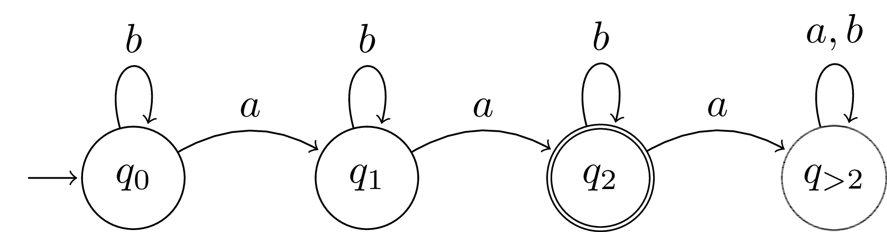
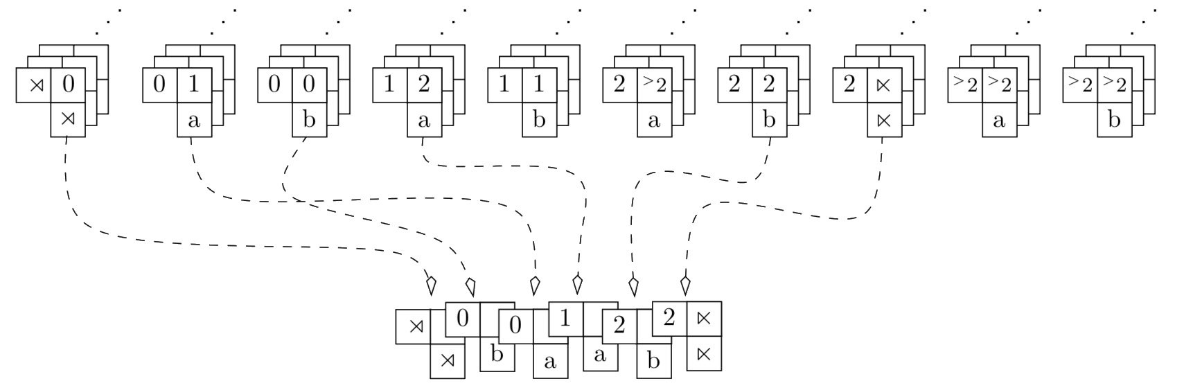
We can think of FSAs as both recognizers and generators, in the same way as we could for strictly-local grammars. Here are some diagrams showing and FSA that recognizes (generates) the language that contains exactly 2 \(a\)’s.

\[\small T=%\langle\ltimes,\ltimes,q_0\rangle, \langle q_0,a,q_1 \rangle, \langle q_0,b,q_0 \rangle, \langle q_1,a,q_2 \rangle, \langle q_1,b,q_1 \rangle, \langle q_1,b,q_1 \rangle, \langle q_2,a,q_{>2} \rangle, \langle q_2,b,q_2 \rangle, %\langle\rtimes,\rtimes,0\rangle, \langle q_{>2},a,q_{>2} \rangle, \langle q_{>2},b,q_{>2} \rangle\]

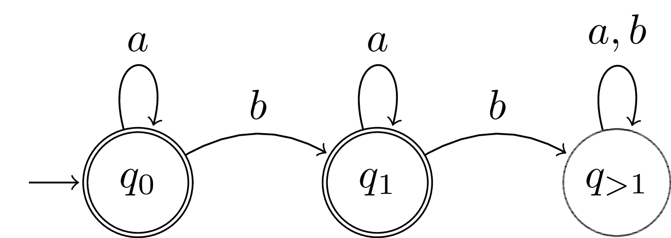
Likewise, it’s easy to see that a FSA can recognize the language $L_{\le1b}$

Regular Languages

An instantaneous description of an FSA \(\mathcal{A}= \langle Q, V, T, q_\rtimes, F_{\ltimes} \rangle\) is a pair \(\langle q, w\rangle\) where \(q \in Q_{\mathcal{A}}\) and \(w \in V_{\mathcal{A}}^*\). It is used to describe the situation where the automaton is in state \(q\) and is reading or generating the input word at the left edge of \(w\) (i.e., \(w\) is the rest of the string). We say an instantaneous description (ID) \(\langle q, w\rangle\) directly computes another ID \(\langle q^\prime, w^\prime \rangle\) with \(\mathcal{A}\), which we write \(\langle q, w\rangle \vdash_{\mathcal{A}} \langle q^\prime, w^\prime \rangle\) if \(w=\sigma w^\prime\) and \(\langle q, \sigma, q^\prime \rangle \in T\). We write \(\langle q, w \rangle \vdash^*_{\mathcal{A}} \langle q^\prime, w^\prime \rangle\) when there is a chain of directly computes relations between individual instantaneous descriptions reaching from \(\langle q, w \rangle\) to \(\langle q^\prime, w^\prime \rangle\) and read this relation as computes.

The formal language \(L(\mathcal{A})\) defined by an FSA \(\mathcal{A}\) is now defined as follows.

\[L(\mathcal{A}) = \{ w \in V^* \mid \langle \rtimes, w \rangle \vdash^*_{\mathcal{A}} \langle q_F, \epsilon \rangle, q_F \in F \}\]

The class of languages for which there exists an FSA is called the regular languages, \(\mathrm{REG}\).

\[\mathrm{REG} = \{L\subseteq V^*\mid \exists \mathcal A \text{ such that } L = L(\mathcal A)\}\]

Another way of defining regular languages is inductively:

• Base cases: \(\varnothing \in \mathrm{REG}\), \(\{\epsilon\} \in \mathrm{REG}\), and \(\{v\} \in \mathrm{REG}\) for $v\in V$
• Inductive step:
  • If $L \in \mathrm{REG}$ then $L^* \in \mathrm{REG}$.
  • And, if $L_1,L_2 \in \mathrm{REG}$ then $L_1\cup L_2\in \mathrm{REG}$ and $L_1\cdot L_2 \in \mathrm{REG}$.
• Nothing else is a regular language.

Regular Languages and Strictly Local Languages

What is the relationship between the regular languages and the strictly local languages? We claim that every strictly local language is a regular language. What do we need to do to prove this?

Recall that a strictly \(k\)-local grammar is a pair, \(\langle V, T \rangle\) where \(V\) is the vocabulary and \(T \subseteq \mathbf{F}_k(\{\rtimes\} \cdot V^* \cdot \{\ltimes\})\). In order to prove that \(\mathrm{SL} \subsetneq \mathrm{REG}\), we must show that we can construct an FSA that recognizes the language of any strictly-local grammar. How can we do this?

The basic idea is simple. Consider \(\mathcal{G}_{\mathrm{SL}}=\langle V_{\mathrm{SL}}, T_{\mathrm{SL}} \rangle\), we construct the following FSA \(\mathcal{G}_{\mathrm{REG}}=\langle Q_{\mathrm{REG}}, V_{\mathrm{REG}}, T_{\mathrm{REG}}, q_\rtimes, F_{\ltimes} \rangle\).

• \(Q_{\mathrm{REG}}\): We add the following states to our FSA. First, for every \(k\)-factor \(f= w_1 \cdots w_{k} \in T_{\mathrm{SL}}\) we introduce a state \(q_{w_1\cdots w_{k}}\), we also introduce the state \(q_{\mathrm{reject}}\) and a distinguished state \(q_{\rtimes}\). Finally, we add a state \(q_{\rtimes \cdots w_{i}}\) for every prefix of any \(k\)-factor in \(T_{\mathrm{REG}}\) of length \(i < k\) that starts with \(\rtimes\).

• \(V_{\mathrm{REG}}\): We set \(V_{\mathrm{REG}}=V_{\mathrm{SL}}\).

• \(T_{\mathrm{REG}}\): First, for each prefix state \(q_{\rtimes \cdots w_{i}}\) with \(i<k\) we add a transition to \(\langle q_{\rtimes \cdots w_{i}}, w^\prime, q_{\rtimes \cdots w_{i}w'} \rangle\), assuming that \(q_{\rtimes \cdots w_{i}w'}\) is either a valid prefix of some factor in our original grammar or a factor in our grammar with \(|{\rtimes}\cdots w_{i}w'|=k\) . We also add a transition \(\langle q_{\rtimes \cdots w_{i}}, w^\prime, q_{\mathrm{reject}} \rangle\) if \(q_{\rtimes \cdots w_{i}w'}\) is not a valid factor or prefix of any factor.

  Next, for each \(k\)-factor \(w_1 \cdots w_{k} \in T_{\mathrm{SL}}\) we introduce the following transition relations: \(\langle q_{w_1 \cdots w_{k}}, w^\prime, q_{w_2 \cdots w_{k} w^\prime} \rangle\) if \(q_{w_2 \cdots w_{k} w^\prime} \in Q_{\mathrm{REG}}\) and \(\langle q_{w_1 \cdots w_{k}}, w^\prime, q_{\mathrm{reject}} \rangle\) if it is not. We also add a transition \(\langle q_{\mathrm{reject}}, w, q_{\mathrm{reject}}\rangle\) for all words \(w\).

• \(F_{\ltimes}\): We set all states \(q_{w_i \cdots \ltimes}\) corresponding to valid factors ending with \(\ltimes\) as accepting states of the machine.

Example

As an example, take the language $(ab)^*\in\mathrm{SL}_2$. Following the above procedure leads to the following FSA for this language: Note that while this procedure will give an FSA for any strictly local language, it does not necessarily give the simplest FSA. It is relatively easy to see that we can simplify the above FSA to the following one, which describes the same language, $(ab)^*$: In this case we were able to take an FSA for our language and find another FSA that describes the same language, while reducing the number of states roughly in half. One question this brings up is whether there is a way to tell whether a given FSA has the minimal number of states required. One way of quantifying this minimal number of states is by the Myhill-Nerode theorem, introduced in the next chapter.

This construction shows the desired property, that we can construct an FSA that recognizes any strictly local language, thus \(\mathrm{SL} \subseteq \mathrm{REG}\). However, we have already seen that \(\mathrm{SL}\) cannot recognize the language \(L_{\le1b}\) (in the chapter Abstract Characterizations). So there are languages that are in REG but not SL. This means that the containment is strict.

\[\mathrm{SL} \subsetneq \mathrm{REG}\]

---

---

← 26 The Backward Algorithm 28 The Myhill-Nerode Theorem →