16 Hierarchical Models
(defn flip [p]
  (if (< (rand 1) p)
    true
    false))

(defn sample-categorical [outcomes params]
  (if (flip (first params))
    (first outcomes)
    (sample-categorical (rest outcomes)
                        (normalize (rest params)))))

(defn score-categorical [outcome outcomes params]
  (if (empty? params)
    (error "no matching outcome")
    (if (= outcome (first outcomes))
      (first params)
      (score-categorical outcome (rest outcomes) (rest params)))))

(defn list-unfold [generator len]
  (if (= len 0)
    '()
    (cons (generator)
    (list-unfold generator (- len 1)))))

(defn normalize [params]
  (let [sum (apply + params)]
    (map (fn [x] (/ x sum)) params)))
Laplacian smoothing, which we saw in Smoothing, is intuitive but it also seems somewhat arbitrary. Why add a constant to each count? Is there a more general framework for understanding what we are doing by adding in pseudocounts to our model?
Researchers have developed many different theoretical frameworks in which one can formalize and study the problem of inductive inference. Although there is no fully general approach to inductive inference, there are two desiderata that come up repeatedly in practice in most applications. First, we would like to choose models in our class that fit the data well. Second, we would like to choose models in our class that are simple or highly generalizable. Many approaches to inductive inference seek to balance these two—often opposing—desiderata against one another. In this chapter, we consider one approach to this problem: the use of prior distributions.
When we come to an inference process, like choosing a good parameterization of our categorical bag-of-words model, we come with prior beliefs. For instance, we may believe that it is unlikely that any vocabulary items will have extremely low probability. Or we may believe that our distribution should be as close to the uniform distribution as possible because it is likely that any sample we see is somewhat skewed from the true underlying distribution over words.
We can encode such beliefs using a prior distribution over the parameters \(\vec{\theta}\). So far, we have been considering the simplex \(\Theta\) to be just the space of possible parameterizations of bag-of-words models. Now, however, we consider \(\Theta\) to be a random variable and we define a distribution over it: \(\Pr(\Theta = \vec{\theta})\).
Given such a distribution over \(\vec{\theta}\) we can define a hierarchical model.
\[\begin{align} \vec{\theta} &&\sim&&& {\color{gray}{\mathrm{somedistribution}(\ldots)}}\\ w^{(1,1)}, ..., w^{(1,n_1)},..., w^{(|\mathbf{C}|,1)}, ..., w^{(|\mathbf{C}|,n_{|\mathbf{C}|})} \mid \vec{\theta} &&\sim&&& \mathrm{Categorical}(\vec{\theta})\\ \end{align}\]We also write this model using probability notation like so.
\[\Pr(\mathbf{C},\vec{\theta}) = \Pr(\mathbf{C}|\vec{\theta})\Pr(\vec{\theta})\]Such a model is called a hierarchical generative model, since it spells out how a corpus is sampled in steps from top to bottom. First we sample a value for \(\vec{\theta}\) and we use this value to sample our corpus.
Distributions on the Simplex
What kinds of distributions could be used for “${\color{gray}{\mathrm{somedistribution}}}$”?
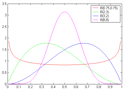
Naturally, it will need to be a distribution on the set of all probability vectors, that is a distribution on the simplex \(\Theta\). We can visualize different distribution on the \(1\)-dimensional simplex like so.
With three dimensional probability vectors we can visualize this using a heat map over the \(2\)-dimensional simplex.
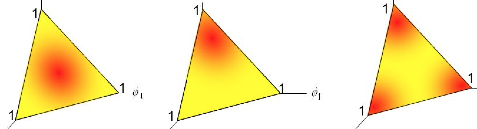
For higher numbers of dimensions, such distributions become difficult to visualize, so it is useful to keep in mind the picture in three dimensions when reasoning about them.
Dirichlet distributions
A very commonly used probability distribution on the simplex is the Dirichlet distribution. The Dirichlet distribution can be defined as follows.
\[p\left(\theta_{1},\ldots ,\theta_{K};\alpha _{1},\ldots ,\alpha _{K}\right)= \frac{1}{B(\vec{\alpha})}\prod _{i=1}^{K}\theta_{i}^{\alpha _{i}-1}\]Where \(B(\vec{\alpha})\) is just the normalizing constant that makes the distribution have a total probability of \(1\). Recall that integration is the continuous analog of summation. In mathematical notation:
\[B(\vec{\alpha})=\int_{\Theta} \prod _{i=1}^{K}\theta_{i}^{\alpha _{i}-1} \,d\vec{\theta}\]Note that here we are using integration from multivariate calculus to “add up” all of the probability mass in the simplex \(\Theta\). For a description of what we mean by this notation, see this note on integrating over the simplex. Using some calculus, it can be shown that
\[B(\vec{\alpha}) =\int_{\Theta} \prod _{i=1}^{K}\theta_{i}^{\alpha_{i}-1} \,d\vec{\theta} =\frac{\prod_{i=1}^{K} \Gamma(\alpha_i)}{\Gamma(\sum_{i=1}^K \alpha_i)}\]where we are using the gamma function \(\Gamma(\cdot)\), which can be thought of as a continuous generalization of the factorial function—in particular, for positive integer values of \(n\), the gamma function is \(\Gamma(n) = (n-1)!\).
So we can write the entire Dirichlet distribution as
\[p\left(\theta_{1},\ldots ,\theta_{K};\alpha _{1},\ldots ,\alpha _{K}\right)= \frac{\Gamma(\sum_{i=1}^K \alpha_i)}{\prod_{i=1}^{K} \Gamma(\alpha_i)} \prod _{i=1}^{K}\theta_{i}^{\alpha _{i}-1}\]The critical thing about the Dirichlet distribution is that the probability that it assigns to \(\vec{\theta}\) is proportional to a term that looks very similar to our categorical likelihood. We will see why this is useful soon.
\[p\left(\theta_{1},\ldots ,\theta_{K};\alpha _{1},\ldots ,\alpha _{K}\right) \propto \prod _{i=1}^{K}\theta_{i}^{\alpha _{i}-1}\]Let’s look at some of the properties of the Dirichlet distribution. First, the mean or center of mass of a Dirichlet distribution is given by \(\frac{\alpha_i}{\sum_{j} \alpha_j}\) for each component \(i\). In other words, the distribution is centered on the probability vector given by renormalizing the pseudocounts.
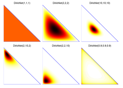
When the values of \(\vec{\alpha}\) are equal to \(1\) the result is the uniform distribution on the simplex. When the values of \(\vec{\alpha}\) are greater than \(1\) the Dirichlet distribution concentrates its mass around the mean of the distribution. The larger the values, the tighter the mass will be concentrated around the mean and the more peaked the distribution will be towards this point.
When the values of \(\vec{\alpha}\) are less than \(1\) (but greater than \(0\)) the probability mass will be “thrown out” from the mean towards the edges of the simplex. The closer to \(0\), the more peaked the distribution will be towards the edges or corners. All of these are illustrated in the following plot.
How can we define a sampler for a Dirichlet distribution? To do this we implement a sampler for another commonly used distribution, the Gamma distribution. We won’t go into how this works, except to note this is another example of the common pattern in probability theory where we build samplers for more complex distributions from simpler distribution (like the Gamma). Many distributions in the so-called exponential family can be built using Gamma distributions.
(defn sample-gamma [shape scale]
  (/ (apply +
  (repeatedly
         shape
	     (fn [] (- (Math/log (rand))))
	    ))
     scale))

(defn sample-dirichlet [pseudos]
  (let [gammas (map (fn [sh]
                     (sample-gamma sh 1))
                pseudos)]
    (normalize gammas)))

(sample-dirichlet (list 1 1 1))
Dirichlet-Categorical Distributions
Now with Dirchlet distribution defined in this way, we can define a new kind of random variable, called the Dirichlet-categorical. This is a single random variable which encapsulates the hierarchical sampling process we defined above. We define the following hierarchical generative model.
\[\begin{align} \vec{\theta} &&\sim&&& \mathrm{Dirichlet}(\vec{\alpha})\\ w^{(1,1)}, ..., w^{(1,n_1)},..., w^{(|\mathbf{C}|,1)}, ..., w^{(|\mathbf{C}|,n_{|\mathbf{C}|})} \mid \vec{\theta} &&\sim&&& \mathrm{categorical}(\vec{\theta})\\ \end{align}\]Or written in probability notation:
\[\Pr(\mathbf{C},\vec{\theta} \mid \vec{\alpha}) = \Pr(\mathbf{C}\mid \vec{\theta}, \vec{\alpha})\Pr(\vec{\theta} \mid \vec{\alpha})\]In fact, given our definition of the hierarchical generative process above, the probability of the corpus \(\Pr(\mathbf{C}\mid \vec{\theta}, \vec{\alpha})=\Pr(\mathbf{C}\mid \vec{\theta})\) doesn’t depend on \(\vec{\alpha}\) once we know \(\vec{\theta}\), that is \(\mathbf{C}\) is conditionally independent of \(\vec{\alpha}\) given \(\vec{\theta}\).
\[\Pr(\mathbf{C},\vec{\theta} \mid \vec{\alpha}) = \Pr(\mathbf{C}\mid \vec{\theta})\Pr(\vec{\theta} \mid \vec{\alpha})\]Notice that the important thing about the Dirichlet-categorical model is that the probability vector \(\vec{\theta}\) is drawn once and reused throughout the whole sampling process over words. How can we write this in Clojure? We need to somehow produce a function which can sample from our vocabulary \(V\) using some random draw of \(\vec{\theta} \sim \mathrm{Dirichlet}(\vec{\alpha})\). One way we can do this using a closure—a function which captures the value of a variable in it’s definition.
(defn make-Dirichlet-categorical-sampler
  [vocabulary pseudos]
  (let [theta
        (sample-dirichlet pseudos)]
    (fn []
      (sample-categorical vocabulary theta))))

(def sample-Dirichlet-categorical
  (make-Dirichlet-categorical-sampler
   '(Call me Ishmael) '(1 1 1)))

(list-unfold sample-Dirichlet-categorical 10)
Scoring a Dirichlet-Categorical
How do we implement a scorer for our hierarchical Dirichlet-categorical model? Now we run into a problem. We can easily score a corpus if we were given a particular value of \(\vec{\theta}\). But now \(\vec{\theta}\) is no longer a parameter of our hierarchical model, it is a random variable. Our joint model is defined with parameter vector \(\vec{\alpha}\). The quantity that we need to compute is \(\Pr(\mathbf{C}|\vec{\alpha})\), but what we have access to (in our hierarchical generative model) is the quantity \(\Pr(\mathbf{C}, \vec{\theta}|\vec{\alpha})\). How do we convert from this joint probability to the desired marginal probability?
Recalling that when we want to remove a random variable from a joint distribution we need to marginalize it away, we see that we need marginalize out \(\vec{\theta}\) using integration.
\[\begin{aligned} \Pr(\mathbf{C}\mid\vec{\alpha}) &= \int_{\Theta} \Pr(\mathbf{C},\vec{\theta}\mid\vec{\alpha}) \,d\vec{\theta}\\ &= \int_{\Theta} \Pr(\mathbf{C}\mid\vec{\theta}) \Pr(\vec{\theta}\mid\vec{\alpha}) \,d\vec{\theta}\\ &= \int_\Theta \left[\prod_{w\in V}\theta_w^{n_w}\right] \left[ {\frac {\Gamma \left(\sum_{w^\prime\in V}\alpha_{w^\prime}\right)} {\prod_{w^\prime \in V} \Gamma(\alpha_{w^\prime})}} \prod_{w \in V}\theta_w^{\alpha_w-1} \right] \,d\vec{\theta}\\ &= {\frac {\Gamma \left(\sum_{w^\prime\in V}\alpha _{w^\prime}\right)} {\prod _{w^\prime \in V} \Gamma(\alpha _{w^\prime})}} \int_{\Theta} \prod_{w \in V}\theta_w^{n_w} \prod_{w \in V}\theta_w^{\alpha_w-1} \,d\vec{\theta}\\ &= {\frac {\Gamma \left(\sum_{w^\prime \in V}\alpha_{w^\prime}\right)} {\prod _{w^\prime \in V} \Gamma(\alpha_{w^\prime})}} \int_{\Theta} \prod_{w \in V}\theta_w^{[n_w+\alpha_w]-1} \,d\vec{\theta}\\ &= {\frac {\Gamma \left(\sum_{w^\prime \in V}\alpha_{w^\prime}\right)} {\prod _{w^\prime \in V} \Gamma(\alpha_{w^\prime})}} {\frac {\prod _{w \in V} \Gamma([n_w+\alpha_w])} {\Gamma \left(\sum_{w \in V}[n_w+\alpha_w]\right)}} \end{aligned}\]This is a complicated expression, but the core idea is that when we wish to know the score of a corpus, and there are latent random variables, such as the variable \(\vec{\theta}\), we must marginalize over these random variables. Note that you can do the integral above without using any calculus just by noting that the following expression holds.
\[\int_{\Theta}\prod _{i=1}^{K}\theta_{i}^{x _{i}-1}\,d\vec{\theta} = \frac{\prod_{i=1}^{K}\Gamma(x_i)}{\Gamma(\sum_{i=1}^K x_i)}\]← 15 Independence, Marginalization, and Conditioning 17 Balancing Fit and Generalization →