29 Determinism and Non-Determinism
In Section Infinite Languages and Recursion, we introduced the notion of non-deterministic choice—an open choice between several options. The distinction between non-determinism and it’s opposite, determinism, is a fundamental one in computer science. A non-deterministic model or algorithm is fundamentally one which can exhibit different behavior on different runs, whereas a deterministic algorithm or model always behaves the same way on the same inputs.
The distinction between determinism and non-determinism arises in the study of many models of computation. For example, it is the basis of the famous question of whether deterministic polynomial time is equivalent to non-deterministic polynomial time (i.e., does P=NP?). We will see other examples later in the book that are relevant for language. In this unit, we will examine our first example if a non-trivial version of this distinction.
In Section Finite-State Automata, we briefly mentioned that our definition of a finite-state automaton was actually the definition of a non-deterministic finite-state automaton, often abbreviated an NFA. Recall that a non-deterministic finite state automaton (NFA) \(\mathcal{A}\) is a five-tuple \(\langle Q, V, T, q_{\rtimes}, F_{\ltimes} \rangle\) where \(Q\) is a set of states, \(V\) is the vocabulary (as usual), \(T\) is the transition relation \(T \subseteq Q \times V \times Q\), \(q_\rtimes \in Q\) is the initial state and \(F_{\ltimes} \subseteq Q\) is a set of accepting states. What makes this definition non-deterministic?
Consider the transition relation \(T\). Since this relation is defined as a subset of \(Q \times Q \times V\) it will allow multiple transitions to different states given the same starting state and same vocabulary item. For instance, consider the NFA below.
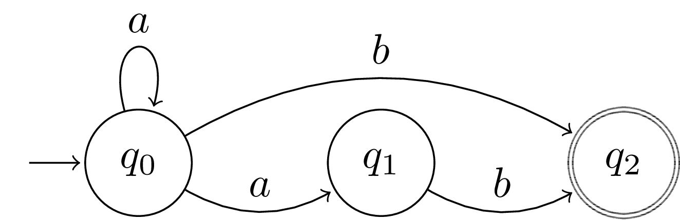
Notice that there are two possible transitions labeled with \(a\) leaving \(q_0\). In other words, both \(\langle q_0, a, q_0\rangle\) and \(\langle q_0, a, q_1\rangle\) are elements of \(T\). If we are to use an NFA to do recognition of strings in a formal language, we will need some way to choose which transitions to take when there is more than one available for a given input.
To make this model deterministic, we merely restrict the transition
relation \(T\) to be a function. That is, we require that for all
transitions \(t=\langle q,\sigma, q^\prime,\rangle \in T\) and
\(t^{\prime}=\langle q, \sigma, q^{\prime\prime}, \rangle \in T\),
\(q^\prime = q^{\prime\prime}\). In other words, there can only be at
most one transition out of each state for a given input symbol.
An NFA with this restriction is referred to as a deterministic finite-state automaton, often abbreviated as DFA. Clearly, every DFA is an NFA, but the set of all possible DFAs forms a strict subset of the set of NFAs. A natural question that arises is whether DFAs have less formal power than NFAs. Does the restriction change the weak generative capacity of the system?
The addition of non-determinism seems intuitively to give the formalism more power. In the case of some formalisms, it does give more power (we will see some later in the course). However for FSAs, surprisingly, non-determinism offers no greater power! In other words, for every NFA, \(\mathcal{N}\) that recognizes formal language \(L_{\mathcal{N}}\) there is a DFA, \(\mathcal{D}\) which recognizes the same language.
How do we prove this. We need to take as input an NFA \(\mathcal{N}\) and output a DFA \(\mathcal{D}\) that recognizes the same language. Let \(\mathcal{N} = \langle Q^\mathcal{N}, V^\mathcal{N}, T^\mathcal{N}, q_{\ltimes}^{\mathcal{N}}, F^{\mathcal{N}}_{\rtimes} \rangle\). The idea of the proof is that we will construct a DFA whose states corresond to subsets of states of \(\mathcal{D}\). First, we set the set of states in our DFA to be equal to the powerset of the set of states in our NFA, that is \(2^{Q^\mathcal{N}}\). Our vocabularies remain the same. We construct our transition function by mapping all \(\mathcal{N}\)-states in our \(\mathcal{D}\)-state to all \(\mathcal{N}\)-states that are reachable using \(T^\mathcal{N}\) when recognizing symbol \(\sigma\). That is, \(\mathcal{D}\)-state \(q\) consists of some subset of \(\mathcal{N}\)-states. We introduce a transition to \(T^\mathcal{D}\), \(\langle q, \sigma, q^\prime \rangle\) where \(q^\prime = \bigcup\limits_{s \in q} \{ s^\prime \mid \langle s,\sigma,s^\prime \rangle \in T^\mathcal{N}\}\). We set our initial state to be \(\{q_{\ltimes}^{\mathcal{N}}\}\), and our set of final states to be any \(q \in 2^{Q^\mathcal{N}}\) such that at least one element of \(q\) is contained in \(F^{\mathcal{N}}_{\rtimes}\).
Let’s prove that these machines recognize the same languages.
\(x \in L_{\mathcal{D}} \implies x \in L_{\mathcal{N}}\)
In this direction, we need to show that a run through the determinized automaton that ends in an accepting state will correspond to a run through the original automaton that ends in an accepting state.
Recall that an instaneous description (ID) is a pair \(\langle q, w\rangle\) where \(q\) is a state and \(w\) is the rest of the string to be recognized. Recall that the directly computes relation \(\vdash_{\mathcal{A}}\) means that automaton \(\mathcal{A}\) can move from the description before to the description after in one step. When there is a chain of directly computes relations between two instaneous descriptions, we use the computes relation \(\vdash^*_{\mathcal{A}}\).
We will show that \(\langle q^\mathcal{D}_{\rtimes}, w\rangle \vdash^*_{\mathcal{D}} \langle r^{\mathcal{D}}, v\rangle \implies (\forall r^{\mathcal{N}} \in r^{\mathcal{D}})[ \langle q^\mathcal{N}_{\rtimes}, w\rangle \vdash^*_{\mathcal{N}} \langle r^{\mathcal{N}}, v\rangle]\) by induction. Since accepting states for \(\mathcal{D}\) are defined as states which contain at least one accepting state in \(\mathcal{N}\), the above condition guarantees that all strings accepted by \(\mathcal{D}\) are accepted by \(\mathcal{N}\)
The base case of our induction is trivial since have defined \(q^\mathcal{D}_{\rtimes} = \{ q^\mathcal{N}_{\rtimes} \}\). For the inductive step, we observe that the transition relation for \(\mathcal{D}\) is defined as taking all of the transitions for \(\mathcal{N}\) out of the current state of \(\mathcal{D}\).
Q. E. D.
\(x \in L_{\mathcal{N}} \implies x \in L_{\mathcal{D}}\)
In this direction, it suffices to show that the \(\langle q^\mathcal{N}_{\rtimes}, w\rangle \vdash^*_{\mathcal{N}} \langle r^{\mathcal{N}}, v\rangle \implies (\exists r^{\mathcal{D}})[ \langle q^\mathcal{D}_{\rtimes}, w\rangle \vdash^*_{\mathcal{D}} \langle r^{\mathcal{D}}, v\rangle \wedge (r^{\mathcal{N}} \in r^{\mathcal{D}})]\). This direction follows by induction and the construction of \(T_\mathcal{D}\).