We saw in the last unit that when we restricted our distributions to just the words that appeared in our toy corpus sample, we got much higher likelihoods. We also saw that the principle of maximal likelihood will favor solutions that put probability mass on smaller numbers of vocabulary items—if that is what appeared in our data sample. This is becaue the the principle of maximum likelihood applied to the categorical BOWs model assigns probability \(\hat{\theta}{}^{\mathrm{ML}}_{w}\) to each word in the vocabulary \(w\) according to the following expression.

\[\hat{\theta}{}^{\mathrm{ML}}_{w} = \frac{n_{w}}{\sum_{w^\prime \in V} n_{w^\prime}}\]

Thus, any word in our vocabulary that does not appear in the training corpus will receive probability \(0\) (i.e., the principle will never incentivize putting probability mass on words that did not appear in the sample).

There is an obvious problem with this approach. Suppose, like in the example we looked at in Maximum Likelihood, that our corpus consists of nothing more than repeated instances of the sentence Call me Ishmael. Under the principle of maximum likelihoood we will set \(\Pr(Call)=\frac{1}{3}\), \(\Pr(me)=\frac{1}{3}\), and \(\Pr(Ishmael)=\frac{1}{3}\). This will provide very good fit to the particular corpus we are looking at \(C\). However, it will not, in general, generalize well to new data. For example, if we tried to use this model to score another, new sentence, such as Call me Fred it would assign this sentence—or any other sentence involving a new word—probability \(0\).

In fact, this is a general problem not just with maximum likelihood estimation, but with many methods of inference which is known as overfitting. Overfitting refers to the phenomenon where we favor hypotheses which are “too close” to the data, and fail to predict the possibility of datapoints which don’t appear in the sample.

More generally, our fundamental goal is to find good models for natural language sentence structure. As we have argued no finite set of sentences is a good model for natural languages like English. Whatever distribution we define over the set of English sentences, must place some probability mass on an infinite set of sentences.

However, any corpus must be finite. As a result, some well-formed sentences (in fact, infinitely many) will be missing from the corpus by accident. A principle of inductive inference—such as the principle of maximum likelihood—is meant to measure the goodness of fit of a model to a finite corpus. A model which fits a corpus well does so by placing more probability mass on strings which appear in the corpus, at the expense of strings which do not appear in the corpus. But not every string that doesn’t appear in a corpus is ill-formed. Some well-formed strings do not appear purely by accident. Thus, inductive principles always risk “paying too much attention” to the particular forms that happen to appear in the corpus, at the expense of well-formed expressions that do not appear—purely by accident.

At the extreme, if we used a model with enough memory capacity, it could simply memorize the exact dataset it was exposed to, assigning probability \(1\) to exactly that set of sentences, and probability \(0\) to every other possible set of sentences. Such a model would have the highest likelihood theoretically possible. But, of course, could never generalize to any new data.

In this unit, we introduce a simple method for improving model generalizability know as smoothing—which is a general term for moving probability mass from observed outcomes to unobserved outcomes. In order to understand smoothing better, it is useful to first consider our space of possible models \(\Theta\) in a bit more detail.

The Simplex: \(\Theta\)

We have been talking about the space of models in the class of categorical BOW models. In this class, our models are indexed or parameterized by probability vectors over \(k\) outcomes. Before talking about smoothing \(\hat{\theta}{}^{\mathrm{ML}}\) or, more generally, about a priori measures on \(\Theta\), it is useful to see how this space can be visualized.

In \(\mathbb{R}^2\), our probability vectors can be visualized as points on the two-dimensional plane. However, probability vectors must contain only probabilities and must sum to \(1\). Thus, the only points in \(\mathbb{R}^2\) which are valid probability vectors fall along a one-dimensional line segment which run between \(\langle 0, 1\rangle\) and \(\langle 1, 0\rangle\)

What about in \(\mathbb{R}^3\)? This is a bit more interesting to visualize and is shown below.

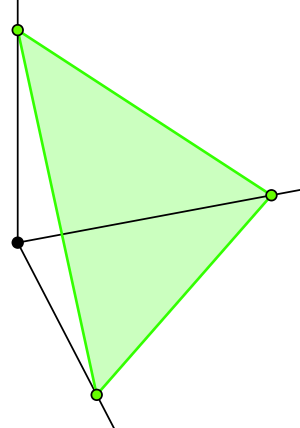
In three dimensions, all the valid probability vectors occur in a two-dimensional triangle anchored at points \(\langle 0, 1, 0\rangle\), \(\langle 1, 0, 0\rangle\), and \(\langle 0, 0, 1\rangle\). In general, all the probability vectors of length \(k\) fall into a \((k-1)\)-dimensional triangle- or pyramid-shaped subspace known as the simplex over \(k-1\) dimensions.

We have seen that the principle of maximum likelihood will choose a probability vector \(\vec{\hat{\theta}}{}^{\mathrm{ML}}\) from \(\Theta\) that have zeros in them. In particular, they have a zero for any position in the vector which corresponds to word that did not appear in the training corpus. If we consider the probability distribution on this vector as a barplot, it will have some high bars and very low bars and won’t be very “smooth.” In terms of the simplex, these distributions appear at the vertices. Smoothing refers to the process of making the bars be a more similar height—in other words, choosing a distribution nearer the center of the simplex, rather than at it’s extremes. How can we do this?

Additive Smoothing

We want to find a way of preventing the maximum likelihood bag-of-words model from overfitting. One way of thinking about this is that we wish to avoid extreme probability distributions that set lots of things to \(0\) and a few things to high probabilities.

A simple way of doing this is Laplace or additive smoothing. To do Laplace smoothing, we add some number \(n\) (often \(1\)) to the count of each word in our vocabulary. Sometimes these numbers are called pseudocounts, we can think of them as an (imaginary) number of times we have seen each word before we observed our corpus \(\mathbf{C}\).

If we let \(\alpha_w\) be the pseudocount associated with word \(w\in V\), then the \(w\)th component of our smoothed maximum likelihood estimator for \(\vec{\theta}\) becomes:

\[{\hat{\theta}}_{w} = \frac{n_{w}+\alpha _{w}}{\sum_{w^\prime \in V}[n_{w^\prime}+\alpha _{w^\prime}]}\]

Laplacian smoothing moves a distribution towards the middle of the simplex, that is, closer to the uniform distribution, \(\theta_w = \frac{1}{\mid V \mid}\) for all \(w\in V\), and prevents any outcome from assigning \(0\) probability to any member of the vocabulary \(V\). Now no finite amount of data can ever take the probability of any word to \(0\), and no sentence over the vocabulary will have probability zero.

---

← 12 Maximum Likelihoood 14 Principles of Inductive Inference →